Operating Plan
Talsim-NG includes an operation model, i.e.it offers the possibility to simulate storage regulation and distribution through defined operating rules. Existing or proposed operating rules need to be converted into a Talsim-NG compatible form.
The model equivalent to conduct of measurements within the river basin is the retrieval of so-called system states of the systems elements. This system states can be processed further and can be connected with mathematical and logical operators (also consecutively) into control clusters. The variety of options and possible connections allows for the representation of almost any desired operating rule. The system state / the control cluster to represent the operating rule is linked to the system element which the rule should be applied to. In case of a reservoir physical boundaries for releases as well as internal dependencies can be implemented. This results in the control logic of the river basin model.
System state
To determine how to represent a system state / system states one might consider the following questions regarding the operation rule to implement:
| subject | Questions about real-world operating rule | Questions about Talsim-NG river basin model | Implementation in Talsim-NG |
|---|---|---|---|
| observed value | On which observed (measured) values are the operating rules based? Which parameters are measured? | Which is the equivalent simulated value, or from which simulated value could the parameter be derived? All simulated values i.e. input-, output- and state variables of the system elements are generally accessible (e.g. discharge, reservoir content, ...). | choose system element and parameter → implement system state |
| spatial reference | At which location ist the observation / measurement made? | Which specific system element (key) can therefor represent the observation / measurement (with which simulated value for system state)? | |
| temporal reference | What is the temporal reference of the observation / measurement? Is the instantaneous value used, a balance or an antecedent value? | Which of the available options in Talsim-NG represents the temporal reference best? | Define objective of the system state and options for value changes respectively |
| transformation | Is the measured value changed subsequently bevor it is included in the operating rule (e.g. unit conversion, weighting function, ...)? | Which function in Talsim-NG can represent the transformation? | Selection and Implementation of the transformation function of the system state |
After these questions regarding the parameter and the location of measurement are resolved satisfactory, a system state can be created. For this system state state attributes can be defined subsequently. The following options are available:
State Attribute Type
Talsim-NG offers the following alternatives to set the type of the system state:
| A | Current Value | uses the current value without any modifications |
| F | Function | value is transformed by means of a function |
| B | Balance (with target) | value is used as discrepancy from target value in % |
| C | Balance (without target) | calculates the balance of the value over several timesteps |
| Z | Objective function | value is the result of an objective function |
| P | Control gauge | currently disabled |
| S | Sum | sum of the state instead of singular value |
Current Value
The option current value uses the simulated value of the current timestep without any modifications:
result = current value of the system state
Function
The option Function also uses the current timestep as time reference, but it includes the possibility to transform the value by means of a function. Since the other options (exception: current value) can be transformed afterwards as well, this will be explained in the next section.
Balance
A balance can be defined as
- an average over the last n time steps (max. 1200)
- a fixed timeframe (start date to end date)
- a constant timeframe (moving average)
- the i-th time step
In the case of Balance(without target), the balance itself is the start value for the subsequent transformation.
In the case of Balance (with target) the discrepancy is used as start value for the Transformation and is calculated as follows:
Discrepancy = ((BALANCE- target value) / target value) * 100
The target value is defined as a constant possibly scaled with an annual pattern.
Sum
Value Modification
Transformation Function
The system states can be transformed additionally by means of a function (exception: Type Current Value). The options include
|
Capacity curve |
|
Fixed annual pattern |
|
Variable annual pattern |
|
Zoning plan / pool-based operating plan |
|
Time-dependent function |
Capacity Curve
The simplest option and the default for any system state that is not treated as current value is the capacity curve. Here the supporting points of a function are entered, according to which the values are transformed. The functions entry value in each case is the system state according to its type (e.g. current value with type function, balance with type balance (without target) or discrepancy (%) with balance (with target)). The function can be interpreted as a step function or interpolated between the supporting points.
If the user chooses not to perform a transformation, the capacity curve can be defined as a 1:1 function. It is important that the entire value range is included, because otherwise the y-value of the first supporting point is used for values smaller than the first supporting point and the y-value of the last supporting point for values bigger than the last supporting point. In addition, the interpolate points option must be set here.
| X-Wert | Y-Wert |
|---|---|
| -10000 | -10000 |
| 10000 | 10000 |
If the user chooses to define constants for the implementation of the operating, it is likewise possible with the option capacity curve:
| X-Wert | Y-Wert |
|---|---|
| 0 | 20 |
| 1 | 20 |
Annual Pattern
In the option annual pattern, a function with one supporting point is defined for various time periods within a year. With a constant annual pattern, the subdivision is done by month, resulting in a total of 12 supporting points. In the case of the variable annual pattern the subdivision is made at any desired date.
For every (temporal) supporting point in the annual pattern values for x and y are declared. Is the system state bevor the transformation smaller than the x value, it is set to zero. Is it equal or bigger than the x value, it is transformed to the y value. The current date / timestamp decides which supporting point is used for the transformation.
Default is that the supporting points are kept constant within each respective time frame. Yet, it is also possible to interpolate over time(???)
Pool-based operating plan
With the option Pool-based operating plan the reservoir storage during a year is subdivided in different zones (pools) each pool is associated with a fixed release level. Hence any amount of increasing release levels is defined and for each defined time period the reservoir storage for each release level is given. However, the option Pool-based operating plan is not restricted to described usage. Generally, any chosen x-value (usually: reservoir storage) can be transformed time-dependent into a y-value (usually reservoir release) via a pool-based operatin plan. The y-values of the supporting points are increasing and identical for every timestep.
By default, the supporting points given by the user are interpreted as step values(?). However, it is possible to interpolate in time and / or between the supporting points of x-/y-values.
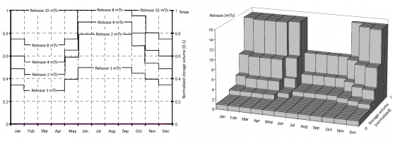
Comparison of a pool-based operating plan in the two- and three-dimensional representation,
Interpretation: constant block (steps)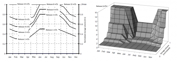
Comparison of a pool-based operating plan in the two- and three-dimensional representation,
Interpretation: linearly interpolated (both in time and between pools)


Time-dependent Function
The time-dependent function is quite similar to the pool-based operating plan, yet more flexible: Among the different time periods, the supporting points of the y-values only have to correspond regaring count, but do not have to be identical in value. Furthermore, they do not necessarily have to be increasing. Hence for each time period any function with any chosen x- and y-value can be definend.
By default, the supporting points given by the user are interpreted as step values(?). However, it is possible to interpolate in time and / or between the supporting points of x-/y-values.
Control Cluster
A control cluster is the linkage of system states and other control clusters with matemathical and logical operators. While a system state represents the condition of a system element, a control cluster can be a unified representation of several system states.
The following operators are available for linkage:
| +/- | Addition and Subtraction |
| ●/÷ | Multiplication and Division |
| <>≤≥ | Comparative Operators |
| mn, mx | Minimum, Maximum |
A control cluster can consist of up to five different system states and/or control clusters. As control clusters can continously be linked further there is no effective limitation regarding number. Any possible combination is feasible. There are no limitations regarding e.g. combination of different values and units. To reach a sensible combination is the obligation of the user.
The system states/ control clusters from which a new control cluster is to be build can be scaled with a factor before linkage with an operator (see Verbindungsfenster).
The control cluster itself, corresponding to the system states, has the state attribute type and can be transformed further with a transformation function (see state attribute something).
Lastly the control cluster can be limited in its value range (see connections).
Control logic
When a rule in a control cluster/ system state is assigned in a way that it represents the desired release from a reservoir or the division from a diversion, the control cluster/ system state is connected with the respective system element. Dependencys among various releases can be implemented either in the definition of a control cluster or using the option internal dependency from the reservoir element.