Simulation of Storage Elements

Navigation
| |

Piecewisely linearized outflow function

The simulation of storage elements is carried out with a newly developed module for the calculation of storage elements whose process functions are linear inbetween nodes. This module is based on the approach of Ostrowski (1992) and is described in detail in Mehler (2000). It allows for the simultaneous solving of the continuity equation for multiple processes without complex iterations and is briefly explained below.

For a storage element whose storage volume depends on several inflow and outflow processes, the continuity equation can be represented as follows:

[math]\displaystyle{ \frac{\mbox{d}S(t)}{\mbox{d}t} = \sum_{j=1}^m Q_{zu,j}(t) - \sum_{i=1}^n Q_{ab,i}(t) }[/math]

with:

S(t) = Storage volume

Qzu,j(t) = Inflow process

Qab,i(t) = Outflow process

m = Number of inflow processes

n = Number of outflow processes

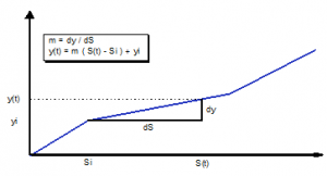
The outflow terms are usually non-linear functions of the storage volume (e.g. outflow from the soil storage with the process functions). These functions are piecewisely linearized.

[math]\displaystyle{ y(t) = A \cdot \left ( \frac{y_{i+1}-y_i}{S_{i+1}-S_i} \cdot (S(t)-S_i) + y_i \right ) }[/math]

with:

[math]\displaystyle{ A = A_1 \cdot A_l \cdot A_{l+1} \cdot \ldots \cdot A_{p-1} \cdot A_p }[/math]

y(t) = Outflow from storage element

S(t) = Storage volume

yi = Outflow value at node i

Si = Storage volume at node i

A = Multiplier of the process variable as a product of all further dependencies

p = Number of additional dependencies

After linearization, a straight line equation which is only dependent on the storage volume can be determined for each process function. The gradient "m" of the line changes from node to node of the process function. Thus, for each function dependent on the storage volume, there is a piecewisely linearized function for the entire range of possible storage volumes. The function itself can be scaled with a factor (A) that is constant for each time step, which summarizes all further dependencies as a product.

The continuity equation can now be reformulated to:

[math]\displaystyle{ \frac{\mbox{d}S}{\mbox{d}t} = \sum_{j=1}^m Q_{z,j}(t) + \sum_{k=1}^m y_{k,i} + \sum_{k=1}^m m_{k,i} \cdot (S(t)-S_i) }[/math]

[math]\displaystyle{ \frac{\mbox{d}S}{\mbox{d}t} = \sum_{j=1}^m Q_{z,j}(t) + \sum_{k=1}^m y_{k,i} + \mbox{C}_2 \cdot (S(t)-S_i) }[/math]

with:

[math]\displaystyle{ \mbox{C}_2 = \sum_{k=1}^m m_{k,i} }[/math]

After multiplying out the brackets the continuity equation becomes:

[math]\displaystyle{ \frac{\mbox{d}S}{\mbox{d}t} + \mbox{C}_2 \cdot S(t) = \mbox{C}_1 }[/math]

with:

[math]\displaystyle{ \mbox{C}_1 = \sum_{j=1}^m Q_{z,j}(t) + \sum_{k=1}^m y_{k,i} + \mbox{C}_2 \cdot S_i }[/math]

This equation is an inhomogeneous first order linear differential equation and has the following solution:

[math]\displaystyle{ S(t) = \frac{\mbox{C}_2}{\mbox{C}_1} \cdot (1-e^{-C_1 \cdot t}) + S_0 \cdot e^{-C_1 \cdot t} }[/math]

with:

[math]\displaystyle{ S_0 = S(t=0) }[/math]

This means that the storage volume can be determined at any time. If, within one time interval, the storage volume reaches the next node, the values of C1 and C2 must be recalculated with the corresponding gradients and intercepts of the piecewise linearized functions at the new node. The simultaneous calculation of the output functions is achieved by inserting the storage volume equation into the respective straight line equation. Generally speaking, the following holds true for the average intensity of all outputs:

[math]\displaystyle{ \bar{y} = \frac{1}{\Delta t} \int_{t=0}^{\Delta t} A \cdot \left [ y_i \cdot S_i + m_i \cdot \left ( \frac{C_2}{C_1} \cdot ( 1 - e^{-C_1 \cdot t} ) + S_0 \cdot e^{-C_1 \cdot t} \right ) \right ] }[/math]

[math]\displaystyle{ \bar{y} = y_i + m_i \cdot \left [ -S_i + \frac{C_2}{C_1} + (1-e^{-C_1 \cdot \Delta t}) \cdot \left ( \frac{S_0}{\Delta t \cdot C_1} - \frac{C_2}{\Delta t \cdot C_1^2} \right ) \right ] }[/math]

With this method, all storage elements whose processes can be described using piecwisely linear functions can be calculated. In Talsim-NG this module is used in the calculation of soil processes, reservoirs and transport reaches.