Berechnungsschema/ Implementierung der Betriebsregeln/en

Navigation
| |

In order to make the principles found accessible for simulation, a suitable mathematical formulation is required.

The previously given order of the principles already gives a structure usable for the mathematical formulation. The main dependency is given by the storage volume. In system hydrology, this kind of dependency is known as a linear single reservoir and can thus be solved to completion. Its principle is based on the assumption that the discharge is always proportional to the amount of water present in the reservoir (storage volume). The proportionality factor k is called the reservoir constant. Taking into account the continuity equation and the reservoir constant, the differential equation of the linear single reservoir is given. However, the reservoir equation is unsuitable for the actual application to storage systems influenced by controls and operation rules. In this case, the discharges are not proportional to the storage volume, and therefore the equation would have to be extended to any number of discharges.

Figure 24: Linearization of a function - section by section

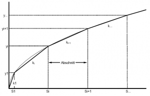
As can be seen from the examples in this chapter, the functional relations between the storage volume and the discharge, used for operating rules, are usually only available as supporting points. The connection of the supporting points gives out the curve progression of a discharge function. A discharge function given in the form of several nodes, e.g. the characteristic curve of a spillway, can be linearly connected between its nodes (or supporting points). The general representation of functions with a linearization, section by section, is given in Figure 24.

One section can be described by:

(2-1)

[math]\displaystyle{ y_{(t)}=y_{i-1}+k_i \cdot (S_{(t)} - S_{i-1}) }[/math]

with

[math]\displaystyle{ S_i \lt S_{(t)} \le S_{i+1} }[/math]

For any number of discharge functions, the equation of a linear single reservoir for a section is:

(2-2)

[math]\displaystyle{ \frac{dS}{dt} = \sum_{z=1}^n Q_z - \sum_{p=1}^m (y_{p,i-1} + k_{p,i} \cdot (S_{(t)} - S_{p,i-1})) }[/math]

with

S : Storage volume

Q_z : Inflow (independent of storage volume).

y_i-1 : Discharge value at supporting point i-1

k : Slope between the supporting points i-1 and i

n : Number of inflows

m : Number of discharges dependent on the storage volume

t : Time

After dividing the equation into a constant part and a part depending on the storage volume S, the known and solvable equation of the linear single reservoir is obtained.

(2-3)

[math]\displaystyle{ \frac{dS}{dt} = \begin{matrix} \underbrace {\sum_{z=1}^n Q_z - \sum_{p-1}^m ( y_{p,i-1} - k_{p,i} \cdot S_{p,i-1} )} \\ C_1=\mbox{konstanter Anteil} \end{matrix} - \begin{matrix} \underbrace {\sum_{p=1}^m (k_{p,i})} \\ C_2=\mbox{von S abhaengig} \end{matrix} \cdot S_{(t)} }[/math]

[math]\displaystyle{ \frac{dS}{dt} = C_1 - C_2 \cdot S_{(t)} }[/math]

As long as the reservoir volumes are within one section Si-1 to Si, the solution to the differential equation is:

(2-4)

[math]\displaystyle{ S(t) = \frac{C_1}{C_2} \cdot \left [ 1 - e^{-C_2} \cdot (t-t_0) \right ] }[/math]

If at least one discharge function exceeds the viewed section, the changes that have occurred up to that point in both the reservoir volumes and the discharges must be registered and C1 and C2 recalculated. With this method, the used time interval - the outer time step - is processed by an arbitrary number of inner time steps depending on the density of the supporting points. The time it takes to undertake a section change can be determined by solving the following equation for t:

(2-5)

[math]\displaystyle{ t_1 = -\frac{1}{C_2} \cdot \ln \left ( \frac{S(t)-\frac{C_1}{C_2}}{S_0-\frac{C_1}{C_2}} \right ) + t_0 }[/math]

Whether a storage volume increases or decreases within the viewed section is to be determined by substituting S(t) by the upper section boundary, whereupon the nearest supporting point of all functions is crucial for the determination of the section boundary. The resulting value t1 determines the following three cases:

1. [math]\displaystyle{ t_1 \gt \Delta t \, }[/math] (outer time step)

   No section change takes place in the considered time interval.

2. [math]\displaystyle{ 0 \lt t_1 \lt \Delta t \, }[/math]

   There is a section change after the time t1. The span between t0 and t1 represents the length of the inner time step.

3. [math]\displaystyle{ t_1 \lt 0 \, }[/math]

   There is no reservoir content increase but a decrease. Instead of the upper section boundary, the lower section boundary must be used and the calculation repeated.

If section changes are observed, the storage volume is known at every time t. Consequently, processes depending on the storage volumes are also known. In general, the development of the curve over time is not required but rather the mean value within one time interval. If equation 2-4 is inserted into equation 2-1 and integrated over the inner time step length, the average process rate in the relevant time interval is obtained.

(2-6)

[math]\displaystyle{ \bar{y} = y_{p,i-1} - k_{p,i} \cdot S_{p,i-1} + k_{p,i} \cdot \left [ \frac{C_1}{C_2} + \left ( 1-e^{-C_2} \cdot (t_1-t_0) \right ) \cdot \left ( \frac{S_0}{(t_1-t_0) \cdot C_2} - \frac{C_1}{(t_1-t_0) \cdot C_2^2} \right ) \right ] }[/math]

After summing up the values of all inner time steps passed through, the average process rate over the entire outer time interval is obtained.

Figure 25: Range-wise linearization of a scaled discharge function

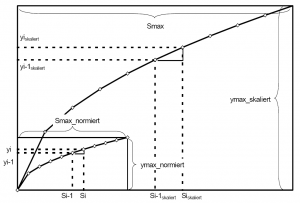
From the principles for the description of operating rules it is evident that a discharge can be dependent on the storage content as well as on other system states. Thus, a one-dimensional dependency - only on the storage content - is no longer given. In such a case, a two- or multi-dimensional relationship exists for the unambiguous determination of a dischrage. If a time dependency is added, the problem is extended by one more dimension. A graphically simple representation is no longer feasible. Likewise the solution described above is not sufficient, since further ones are added to the dependence on the reservoir contents. Both for reasons of clarity and a suitable mathematical formulation, it is desirable to convert all dependencies back into a one-dimensional relationship without loss of information. This is achieved by scaling the discharge functions relationship. A scaling is possible for the discharge (y-axis) as well as for the reservoir content (x-axis).

After introducing the scaling factors, the result for a scaled section of a function is:

(2-7)

[math]\displaystyle{ y_{(t)}^s = y_{i-1} \cdot y_{\mbox{faktor}} + k_i \cdot \frac{y_{\mbox{faktor}}}{x_{\mbox{faktor}}} \cdot \left ( S_{(t)} \cdot x_{\mbox{faktor}} -S_{i-1} \cdot x_{\mbox{faktor}} \right ) }[/math]

[math]\displaystyle{ y_{(t)}^s = y_{i-1}^s + k_i^s \cdot \left ( S_{(t)}^s - S_{i-1}^s \right ) }[/math]

To calculate the delivery function scaled with external system states, proceed analogously to the above method. Here xfactor corresponds to the maximum reservoir content and yfactor corresponds to the scaling factor from the external system state or state group. It is assumed that the factors remain constant during the external time interval. The sum of the integrations over the internal time loop divided by the external time step provides the final output value.

(2-8)

[math]\displaystyle{ \bar{y} = y_{\mbox{faktor}} \cdot \left [ y_{p,i-1} - k_{p,i} \cdot S_{p,i-1} + \frac{1}{x_{\mbox{faktor}}} k_{p,i} \cdot \left [ \frac{\mbox{C1}^s}{\mbox{C2}^s} + \left ( 1 - \mbox{e}^{-\mbox{C2}^s \cdot \left ( t_1 - t_0 \right )} \right ) \cdot \left ( \frac{S_0 \cdot x_{\mbox{faktor}}}{(t_1 - t_0) \cdot \mbox{C2}^s} - \frac{\mbox{C1}^s}{(t_1 - t_0) \cdot {\mbox{C2}^s}^2} \right ) \right ] \right ] }[/math]

The computation of a rangewise linear memory with arbitrarily many inputs and outputs has been described by Ostrowski (1992). This solution was extended to include scaling of both the X and Y axes .

In summary, a reservoir can have any number of uses. For each usage, there is a function dependent on the reservoir content, which must remain constant within an external time step, but can be changed from time step to time step (time dependency). In addition, these functions can be scaled differently for each time step by external dependencies via factors. Prerequisite for the scaling are constant factors during the time step. The calculation process is independent of the time step, since it is decomposed according to the section crossings into arbitrarily many internal time steps. This means that the method is suitable for a wide variety of time intervals and produces results that are true to the volume. Thus, both a flood event with a time step of a few minutes and a long-term simulation with daily values or even larger time intervals can be used. The only decisive factor is that all discharge functions are defined over a sufficient number of grid points.