Sub-Basin

The simulation of natural catchment areas requires the determination of load generation, flow branching and runoff concentration. The methods of calculation used are described below.
Load Generation
The load formation describes the determination of precipitation for the considered catchment area. Only one precipitation is used per catchment area. If there are several precipitation stations in the catchment area, it is useful to divide the area into several system elements 'catchment area', until only one precipitation can be assigned to each element.
Runoff generation of paved/unpaved surfaces
The runoff generation determines the effective precipitation from the rainfall. From this, the components surface runoff, infiltration, evaporation and interflow are derived. A snow calculation is performed at temperatures below zero °C and is based on the Snow-Compaction-Method. Regarding the algorithms of the method, reference is made to the relevant literature. The natural process from precipitation to runoff is divided into individual phases for the mathematical simulation. In the runoff generation phase, the precipitation (system load) is divided into the "effective precipitation" directly reaching the runoff, and the losses not affecting the runoff (moistening, trough, evaporation and infiltration losses). Therefore, this phase is also called load distribution. The resulting mathematical equation for the momentary load distribution is written as follows:
[math]\displaystyle{ N_W(t) =N(t) -VP(t) -I(t) - \frac{dO}{dt} - \frac{dS}{dt} }[/math]
with:
| [math]\displaystyle{ N_W }[/math]: | Runoff-effective precipitation |
| [math]\displaystyle{ N }[/math]: | Precipitation |
| [math]\displaystyle{ VP }[/math]: | Potential evaporation |
| [math]\displaystyle{ I }[/math]: | Infiltration into the floor area |
| [math]\displaystyle{ O }[/math]: | Surface water supply |
| [math]\displaystyle{ S }[/math]: | Snow storage |
In the following, the terms used in the equation and their calculation are explained in detail.
Precipitation N(t)
The precipitation data must be added to the simulation model in the form of rainfall series. In principle, it is irrelevant whether the precipitation series is a block rain, a model rain, a measured natural rain, a rain spectrum or a long-time rain series. Depending on the objective of the simulation calculation the appropriate load has to be selected. The rainfall series are either taken from the time series management of Talsim-NG or are generated, in case of applying a short term forecast, by entering a rainfall duration, a precipitation height and the choice of a rain model directly before a simulation.
Evaporation VP(t)
Evaporation has a double effect on the formation of runoff. On the one hand, the initial conditions in the catchment area (wetting and trough filling on the surface as well as limiting soil moisture on permeable surfaces) are a result of the evaporation taking place before the considered precipitation event. On the other hand, the precipitation to be calculated, which affects runoff, is reduced by the amount of the current evaporation rate. The potential (energetically possible) evaporation VP is very different in time and place and is hardly accessible for an exact calculation. From evaluated measurements of 20 stations, mean values of these stations are presented as histogram. The following compensation function was determined /BRANDT, 1979/.
[math]\displaystyle{ VP=(0.96+0.0033 \cdot i) \cdot \sin\frac{2\pi}{365}(i-148)+158 }[/math]
with:
| [math]\displaystyle{ i }[/math]: | current day of the outflow year |
| [math]\displaystyle{ i=1 }[/math]: | November 1 |
The total annual potential evaporation height is 642 mm. If no measured evaporation values are available, this normalized annual potential evaporation can optionally be used to calculate the current evaporation. If the selected calculation time interval is less than one day, the potential evaporation for each calculation time interval is finally determined by means of the displayed daily variation. If the calculation interval is less than 1 day, the daily course is not taken into account.
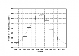
Year of potential evaporation after /BRAND, 1979/
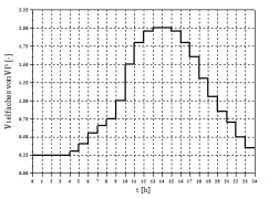
Daily rate of potential evaporation as a multiple of the mean daily evaporation


Surface water supply (sealed area portion)
In the case of sealed surface portions, snow supply and infiltration can be neglected, so that the balance equation is simplified as follows:
[math]\displaystyle{ N_W(t)=N(t)-VP(t)-\frac{dO}{dt} }[/math]
the surface water supply change [math]\displaystyle{ dO/dt }[/math] represents the wetting of the surface as well as the filling and emptying (by evaporation) of the troughs.

The following standard value [math]\displaystyle{ BV }[/math] is used as wetting loss for sealed surfaces.
[math]\displaystyle{ BV = 0.5 \mbox{ mm} }[/math]
The trough loss (MV) is specified by the user. The standard and simultaneously maximum value in the model is 4 mm. The trough loss represents the average value for an sloping surface. However, since the troughs are not evenly distributed and, as experience shows, drainage begins before the complete filling of the troughs has been reached everywhere, it is assumed that
- 1/3 of the sealed surface has a reduced trough loss of 1/3-MV
- 1/3 of the sealed area the average trough loss of 3/3-MV
- 1/3 of the sealed surface has an increased trough loss of 5/3-MV
has. Therefore, runoff already occurs when the precipitation reduced by the evaporation rate exceeds the wetting loss and 1/3 of the trough loss (in case of dry history). The assumptions above are schematically sketched in the following figure.
The runoff coefficient of the sealed surfaces (after covering the initial losses) is set at [math]\displaystyle{ \Psi = 1 }[/math]. When determining the sealed surface of a subcatchment area, it must be taken into account that not all paved or sealed surfaces actually drain into a sewer system. The continuous provision of the wetting and trough losses is achieved by continuous balancing of these reservoirs and evaporation.
Surface water supply (unsealed area)
The surface water supply is calculated by balancing a loss reservoir depending on the selected runoff generation approach. Details can be found in the following sections on the calculation of infiltration or runoff-effective precipitation.
Infiltration or runoff-effective precipitation I(t), NW(t)
In the case of permeable surfaces, infiltration into the soil cannot be neglected, since this has a decisive influence on the runoff. For the calculation three approaches were implemented in the model:
- Constant discharge coefficient [math]\displaystyle{ \Psi }[/math]
- Event-specific discharge coefficient based on the Soil-Conservation-Service (SCS) method
- Soil moisture simulation
Constant discharge coefficient Ψ
If a [math]\displaystyle{ \Psi }[/math] value is given, the remaining part of the precipitation in the ratio of the runoff coefficient [math]\displaystyle{ \Psi }[/math] is added to the runoff after covering the initial losses (wetting and trough loss), independent of the history and characteristics of the precipitation. If possible, this approach should be avoided, since the process of runoff formation is only roughly simplified.
Event-specific discharge coefficient based on the Soil-Conservation-Service (SCS)
If a CN value is given that is dependent on the soil type and land use (see /DVWK, 1991/), a prehistoric initial loss as well as a prehistoric relationship of the runoff coefficient from the amount of precipitation accumulated up to the time under consideration can be formulated /Zaiss, 1987/; i.e. the runoff coefficient increases with increasing precipitation in the course of the event. The quantification of the prehistory is based on the 21-day-precipitation index [math]\displaystyle{ VN }[/math]
[math]\displaystyle{ V_N=\sum_{j=1}^21 C(j)^j \cdot hN_j }[/math]
with:
| [math]\displaystyle{ hN_j }[/math]: | Precipitation height of the j-th previous day |
| [math]\displaystyle{ C(j) }[/math]: | Factor describing the influence of the j-th previous day |
The season impact is represented by a yearly variation of the factor C.
[math]\displaystyle{ C=0.05 \cdot \sin\frac{2\pi}{365}(i+0.75)+0.85 }[/math]
with:
| [math]\displaystyle{ i }[/math]: | current day of the outflow year |
As a result, the value C ranges between 0.8 < C < 0.9. This ensures that different rainfall indices are calculated for the same amount of rainfall at different times of the year and therefore a changed willingness to flow is taken into account. Depending on the prehistory quantified in this way, a current discharge coefficient can be calculated using the CN values specific to the area and valid for average prehistory conditions. The following figure shows for different CN-values how the current discharge coefficient changes depending on the prehistory. Since the runoff readiness of a catchment area changes in the course of a rainfall event due to soil moisture, the runoff coefficient is also adjusted during an event as a function of the cumulative precipitation height.
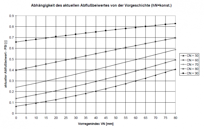
Dependence of the discharge coefficient on the previous history
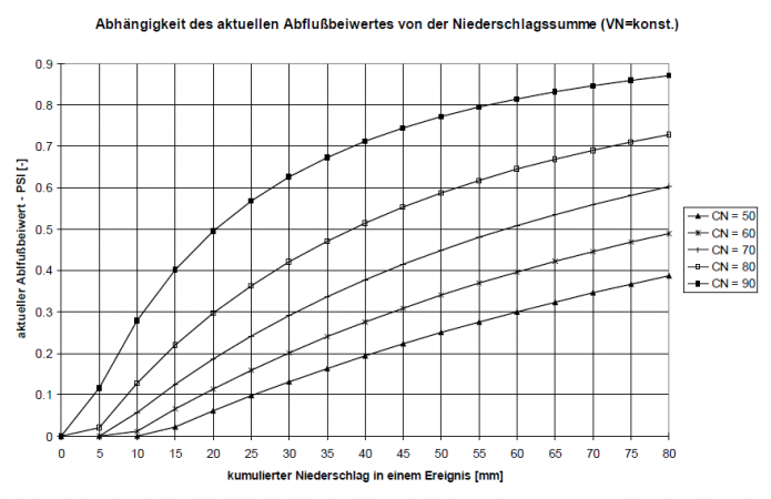
Dependence of the runoff coefficient on the cumulative precipitation sum


Soil Moisture Simulation
Land use
Bei der Anwendung der Bodenfeuchtesimulation ist die Angabe von Landnutzungen notwendig. Aus den Angaben zur Landnutzung wird die Durchwurzelungstiefe benötigt, um die Dicke der Durchwurzelungsschicht zu ermitteln. Weitere Parameter der Landnutzung, die zur Berechnung der Interzeption und der Transpiration dienen, sind:
- Wurzeltiefe
- Bedeckungsgrad
- Jahresgang des Bedeckungsgrades
- Blattflächenindex
- Jahresgang des Blattflächenindexes
Die Angabe von Haude-Faktoren zur besseren Berücksichtigung der Verdunstung je Landnutzung sind über Eingabe von Jahresgängen beliebig möglich und können den gewünschten Landnutzungen zugeordnet werden.
Soil type/ Soil texture


The soil moisture simulation is based on a non-linear calculation of the individual soil horizons. The soil is divided into different horizons (layers). Each layer is calculated and compared with the layers below or above (if available). The following soil physical parameters are used as parameters for the soil moisture calculation:
- Wilting point (WP)
- Field capacity (FK)
- Total pore volume (GPV)
- Saturated conductivity (kf value)
- Maximum infiltration capacity (Max.Inf.)
- Maximum rate of capillary suction (Max.Cap.)
- Assignment to a soil type: sand, silt, clay
Die mögliche Anzahl der Bodenschichten läuft von minimal einer bis maximal sechs. Die Erfahrung zeigte, dass die besten Ergebnisse mit einer Aufteilung in drei Schichten erzielt werden konnten. Aus diesem Grund werden die eingegebenen Schichten programmintern immer in drei Horizonte unterteilt.
- Infiltrationsschicht (Standarddicke [cm] = 20)
- Durchwurzelte Schicht (Mindestdicke [cm] = 5)
- Transportschicht (Mindestdicke [cm] = 5)
Die Berechnung der neuen Bodenkennwerte für die programmintern verwendeten Schichten erfolgt durch eine Gewichtung entsprechend den vorgegebenen original Dicken der Schichten. Im Fall der gesättigten Leitfähigkeit läuft die Berechnung nach dem Prinzip der Erhaltung der Kontinuität der Strömung ab. Bei senkrechter Strömung soll aufgrund der Kontinuität der Strömung die Geschwindigkeit v bei gegebener Durchflussmenge in einer programminternen Schicht denselben Wert besitzen. Damit ist das hydraulische Gefälle nicht mehr konstant.
[math]\displaystyle{ kf_V=\frac{\sum_{i=1}^n d_i}{\sum_{i=1}^n \frac{d_i}{k_i}} }[/math]
mit:
| [math]\displaystyle{ d_i }[/math]: | anteilige Schichtdicke der jeweiligen Original-Schicht [mm] |
| [math]\displaystyle{ k_i }[/math]: | gesättigte Leitfähigkeit der jeweiligen Original-Schicht [mm/h] |
| [math]\displaystyle{ kf_V }[/math]: | gesättigte Leitfähigkeit der programmintern verwendeten Schicht [mm/h] |

Auf der Basis der bereichsweisen linearen Abbildung der die Bodenfeuchte beeinflussenden Prozessfunktionen Infiltration, aktuelle Verdunstung (Evaporation + Transpiration), Perkolation, Interflow und Kapillaraufstieg wird für eine Bodenschicht die Wasserbilanzgleichung gelöst. Die Eingangsgröße für die Evaporation und Transpiration ermittelt sich aus der potentiellen Verdunstung. Die zu lösende Gleichung ist:
[math]\displaystyle{ \frac{dBF(t)}{dt}=Inf(t)-Perk(t)-Eva_{akt}(t)-Trans_{akt}(t)-Int(t)+Kap(t) }[/math]
mit:
| [math]\displaystyle{ BF(t) }[/math]: | aktuelle Bodenfeuchte |
| [math]\displaystyle{ Inf(t) }[/math]: | Infiltration in den Boden |
| [math]\displaystyle{ Perk(t) }[/math]: | Perkolation (Durchsickerung) |
| [math]\displaystyle{ Eva_{akt}(t) }[/math]: | aktuelle Evaporation |
| [math]\displaystyle{ Trans_{akt}(t) }[/math]: | aktuelle Transpiration |
| [math]\displaystyle{ Int(t) }[/math]: | Interflow |
| [math]\displaystyle{ Kap(t) }[/math]: | Kapillaraufstieg |

Infiltration, Perkolation, Evaporation, Transpiration, Interflow und Kapillaraufstieg sind von der aktuellen Bodenfeuchte abhängig. In der Simulation wird diese Abhängigkeit durch folgende Funktionsverläufe beschrieben.
[math]\displaystyle{ Inf(BF(t))=a_v \cdot \left(GPV-BF(t) \right)^{1.4}+k_f }[/math] (Ansatz nach HOLTAN)
[math]\displaystyle{ Perk(BF(t)) = \begin{cases} 0, & BF(t)\le f_{PK} \cdot nFK + WP \\ k_f \cdot \left(\frac{BF(t)-(f_{PK} \cdot nFK +WP)}{GPV-(f_{PK} \cdot nFK +WP)} \right)^{exp,PK}, & BF(t)\gt f_{PK} \cdot nFK + WP \end{cases} }[/math]
- (mod. Ansatz nach /OSTROWSKI, 1992/)
[math]\displaystyle{ Eva(BF(t)) = \begin{cases} 0, & BF(t)\le WP \\ f_{Eva} \cdot \left(\frac{BF(t)-WP}{GPV-WP} \right)^{exp,PK}, & BF(t)\gt WP \end{cases} }[/math]
[math]\displaystyle{ Trans(BF(t)) = \begin{cases} 0, & BF(t)\le f_{Trans} \cdot nFK + WP \\ f_{Trans} \cdot \left(\frac{BF(t)-(f_{Trans} \cdot nFK +WP)}{GPV-(f_{Trans} \cdot nFK +WP)} \right)^{exp,PK}, & BF(t)\gt f_{Trans} \cdot nFK + WP \end{cases} }[/math]
mit:
| [math]\displaystyle{ a_v }[/math]: | Infiltrationsfaktor nach HOLTAN (in Talsim-NG [math]\displaystyle{ a_v=1 }[/math] |
| [math]\displaystyle{ k_f }[/math]: | Durchlässigkeitsbeiwert des gesättigten Bodens |
| [math]\displaystyle{ nFK }[/math]: | nutzbare Feldkapazität ([math]\displaystyle{ nFK=FK-WP }[/math]) |
| [math]\displaystyle{ WP }[/math]: | Welkepunkt |
| [math]\displaystyle{ FK }[/math]: | Feldkapazität |
| [math]\displaystyle{ GPV }[/math]: | gesamtes Porenvolumen |
| [math]\displaystyle{ f_{PK} }[/math]: | bodenabhängiger Skalierungfaktor der Perkolationsfunktion |
| [math]\displaystyle{ exp,PK }[/math]: | bodenabhängiger Krümmungsparameter der Perkolationsfunktion |
| [math]\displaystyle{ f_{Eva} }[/math]: | bodenabhängiger Skalierungsfaktor der Evaporationsfunktion |
| [math]\displaystyle{ f_{Trans} }[/math]: | bodenabhängiger Skalierungsfaktor der Transpirationsfunktion |
| [math]\displaystyle{ exp,Trans }[/math]: | Krümmungsparameter der Transpirationsfunktion |
Die Programmparameter werden intern berechnet. Der Anwender muss lediglich die Bodenkennwerte kf, WP, FK und GPV angeben. Die Berechnung der Bodenprozesse erfolgt mit einem neuentwickelten Baustein zur Simulation von Speichern.
Elementarflächen
Wird mit der Bodenfeuchtesimulation die Abflussbildung berechnet, wird gleichzeitig das Elementarflächenkonzept angewandt. Ein Einzugsgebietselement wird dabei in beliebig viele hydrologisch homogene Flächen unterteilt, d.h. Flächen gleichen Bodentyps und gleicher Landnutzung. Für jede Elementarfläche gilt genau eine Zuordnung von Landnutzung und Bodentyp. Die aus einer Elementarfläche resultierende Wassermenge wird am Elementausgang angesetzt, d.h. alle Elementarflächen geben unabhängig ihrer Lage im Einzugsgebiet Wasser mit der gleichen zeitlichen Verzögerung ab.
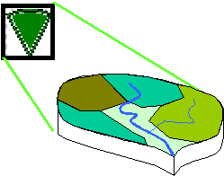
Aufteilung eines Einzugsgebietselementes in Elementarflächen
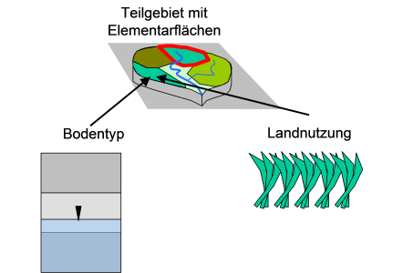
Zuordnung von Bodentyp und Landnutzung zu Elementarflächen


Abflusskonzentration
Die Abflusskonzentration bestimmt die Verzögerung des Oberflächenabflusses aus dem Einzugsgebiet. Es wird eine Parallelspeicherkaskade mit drei Speichern für unbefestigte und eine Kaskade für befestigte Flächen benutzt. Der Abfluss der Komponenten Interflow und Grundwasser wird über einen linearen Einzelspeicher verzögert an den Elementausgang abgegeben.
