Talsim-NG includes a storage operation model, i.e. it offers the possibility to simulate storage regulation and distribution through defined operating rules. Existing or proposed operating rules need to be converted into a Talsim-NG compatible form.
The model equivalent to conducting measurements within the river basin is the retrieval of so-called system states of the system elements. Further, these system states are processed and connected to mathematical and logical operators (also consecutively) into virtual states. The variety of options and possible connections allows for the representation of almost any desired operating rule. The element/ virtual state representing the operating rule is linked to the system element to which the rule should be applied to. In the case of a storage, physical boundaries for releases as well as internal dependencies can be implemented. The result is the control logic of the river basin model.
System States
In Talsim, an Element State represents a calculated internal quantity of a System Element at each simulation time step. These values reflect the current condition of the element — such as precipitation, soil moisture, or baseflow for a Sub-Basin — and can be stored and referenced at specific temporal points (e.g. current value, value from a previous time step, or a moving average). Element States are often used to define operating rules, either directly or as part of more complex logic. When multiple Element States are combined and transformed, they form Virtual States, which support more advanced rule definitions based on multiple conditions or observations.
State Type
Talsim offers the following types of system state attributes:
|
The option current value uses the simulated value of the current time step without any modifications:
result = current value of the system state
|
|
The option function also uses the current time step as time reference, but it includes the possibility to transform the value by applying a function. As the values from this option and all the following options (current value is the only exception) can be transformed, the general transformation process will only be explained in the next section.
|
|
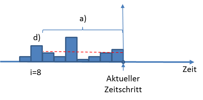
A balance can be defined as
a.an average over the last n time steps (max. 1200)
b.a fixed timeframe (start date to end date)
c.a constant timeframe (moving average)
d.the i-th time step
 Choices when defining a balance In the case of Balance (without target), the balance itself is the initial value for the subsequent transformation.
In the case of Balance (with target) the discrepancy from the target value is used as the initial value for the transformation and is calculated as follows:
Discrepancy = ((BALANCE- target value) / target value) * 100
The target value is defined as a constant possibly scaled with an annual pattern.
|
|
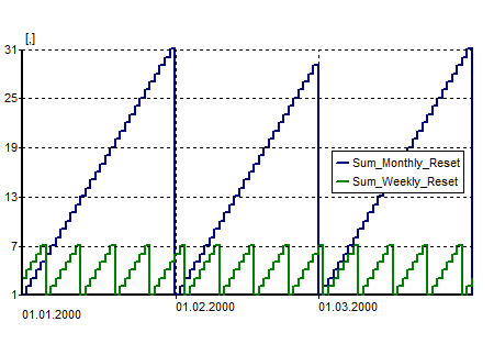
A Sum adds up the past State values up to the current time step. At every Refresh interval the Sum gets reset starting the cumulative sum from zero.

|
With the default setting of the Refresh interval to Each time step the output of Sum equals the output of function thus is not effective.
Change the Refresh interval to activate the computation of Sum.
|

|
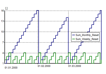
Sum only adds up the values, it is not an integral. A change in the time step will change the results of Sum.
|

|
If the Refresh interval does not lie exactly on a time step, Sum will not be reset exactly at the refresh interval, but at the next time step.
|
 Example for State type Sum: State before Sum is 1. Time step is 1 day. |
 Example for State type Sum: State before Sum is 1. Time step is 2 days. |
|
Transformation Function
The system states are additionally transformed by a function (exception: current value).
The entry value for the transformation depends on the state type (e.g. balance for type balance). First the operations demanded by the state type are computed, then the transformation by the function takes place.
In the following all transformation options are listed:
|
The simplest transformation function and the default for any system state type other than current value is the capacity curve.
The capacity curve consists of supporting points (x, y) defined by the user.

|
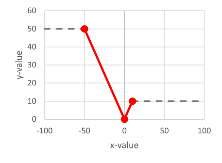
The option Interpolation of points changes the interpretation of the function.
If checked, the function is interpolated between the supporting points, if unchecked it is interpreted as a step function.
Make sure you have this option checked or unchecked as needed.
|
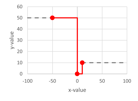
Example function for visualizing the two different interpolation options Interpolation of points checked/unchecked:
x-value
|
y- value
|
-50
|
50
|
0
|
10
|
10
|
10
|
|
 Interpretation of example function: Interpolation of points checked |
 Interpretation of example function: Interpolation of points unchecked |

|
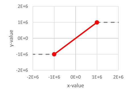
Outside the defined range the function is extrapolated to be constant:
Values below the x-value of the first supporting point x1 become the y-value of the first supporting point y1, values above the x-values of the last supporting point xn become the y-value of the last supporting point yn.
Make sure to include the entire expected data range into the function definition, unless the constant extrapolation is what you need.
|
Example function for visualizing the extrapolation outside the defined range:
x-value
|
y- value
|
-50
|
50
|
0
|
10
|
10
|
10
|
|
 Outside the defined range functions are kept constant to the y-value of the closest supporting point (grey dashed line). |

|

|
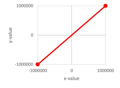
If you don't need a transformation, define the capacity curve as a 1:1 function.
Make sure that the entire expected value range is included.
Check the option Interpolation of points.
|

|
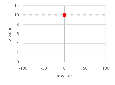
To create a constant, define a function with the same y-values for all the supporting points.
|
|
|
With the option annual pattern, a function with one supporting point is defined for each chosen time period within one year. With a constant annual pattern, the division of the year into time periods is undertaken by month, resulting in a total of 12 supporting points. With a variable annual pattern, the division of the year into time periods is undertaken at the desired dates.
For each (temporal) supporting point, values for x and y are entered. If, before the transformation, the system state value is smaller than the x-value, it is set to zero. If it is equal to or bigger than the x-value, it is transformed to the y-value. Every current date / time stamp constitutes which respective supporting point is then used for the transformation.
By default, the supporting points are kept constant within each time frame. Yet, it is also possible to linearly interpolate over time.
|
|
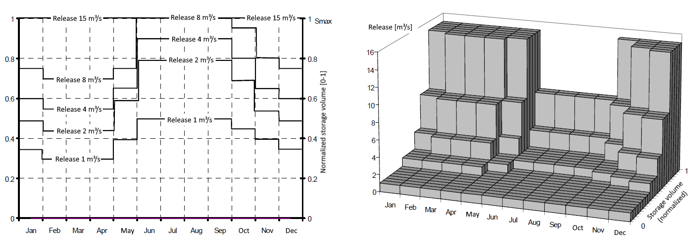
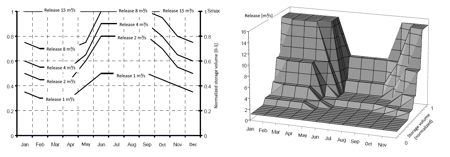
With the option zoning plan, the storage volume during a year is divided into different zones, where each zone is associated with a fixed release level. Hence, for each defined release level and for each fixed time period the specific storage volumes are entered. However, the option zoning plan is not restricted to this use. Generally, any chosen x-value (usually: storage volume) can be transformed into a y-value (usually: storage releases) via a zoning plan. The y-values of the supporting points need to be ascending.
By default, the entered supporting points of the zoning plan are interpreted as blocks, thus they are kept constant along the time-axis and the x-axis until the next supporting point. However, it is also possible to linearly interpolate in time and / or between the supporting points of x-/y-values.
 Comparison of a zoning plan in the two- and three-dimensional representation,
Interpretation: constant block (steps)  Comparison of a zoning plan in the two- and three-dimensional representation,
Interpretation: linearly interpolated (both in time and between x/y-supporting points) |
|
The time-dependent function acts similar to the zoning plan, yet is more flexible: For different periods, the supporting points of the y-values only need to correspond regarding their number but do not have to be identical in value. Furthermore, they do not necessarily have to be ascending. Hence, one picks a user-defined function with individual x- and y-values.
By default, the entered supporting points are interpreted similarly to a step function, but in blocks. However, it is also possible to linearly interpolate over time and / or between the supporting points of x-/y-values.
|
Refresh Interval
This Option allows to set at which time steps the State should be computed, thus a change in its value is allowed. There are three options available. The State will be refreshed:
|
This is the default option. With this option the value of the State is refreshed each time step. No further input is required.
|
|
A daily, a weekly and an annual pattern can be connected to determine at which time steps the State should be refreshed. Talsim refreshes the value of the State always when the product of the patterns is a value > 0.
|
|
With this option the value of the State value is refreshed at a regular time interval, defined as a multiple of the common time units (between minutes and years). The reference date (in the format DD.MM.YYYY hh:mm) serves as a reference point for all the future and former time steps.
|

|
In the case of the State type Sum, the interpretation of the Refresh Interval is a little different: With the Option Sum, the State does get refreshed every time step but it is reset at the Refresh Interval thus starting the cumulative sum from zero again. If the Refresh Interval is left as the default option Each time step the type Sum is just doing the same as the type Function.
|
Options for Linking States
A Virtual State is the combination of Element States and/or other Virtual States using mathematical and logical operators.
The following operators are available for combining States into a new Virtual State:
+/- Addition and subtraction
●/÷ Multiplication and division
<>≤≥ Comparative operators
mn, mx Minimum and maximum
A single Virtual State can combine up to five different States. As Virtual States themselves be linked to create new Virtual States, there is virtually no limit to the number of States that can be combined. There are no restrictions regarding e.g. the combination of different values and units. It is the user's responsibility to achieve reasonable combinations.

|
There are no restrictions regarding the combination of States with different quantities and units.
Senseless combinations are possible and will not result in warnings.
Make sure to get reasonable combinations by converting units using any of the scaling options available.
|
When building new virtual states, the connected system states/control clusters can be scaled by a factor before using the operator for combination.
The control cluster itself, just like the system states, has a system state attribute and can be transformed further with a transformation function (see state attribute window).
Lastly, the control cluster can be limited in its value range (see connections).
Control Logic
If a rule in a control cluster/ system state is assigned in a way that it represents the desired release from a storage or it describes the division from a diversion, the control cluster/ system state is connected to the respective system element. Dependencies between various releases can be implemented either via the definition of a control cluster or using the option internal dependency from the storage element.

