Einzugsgebiet/en: Unterschied zwischen den Versionen
Ferrao (Diskussion | Beiträge) (Die Seite wurde neu angelegt: „with: {|style="margin-left: 40px;" |<math>hN_j</math>: || Precipitation height of the j-th previous day |- |<math>C(j)</math>: || Factor describing the influen…“) |
(Die Seite wurde neu angelegt: „====Compensation functions==== The following compensation functions according to Brandt are used to distribute entered annual values for evaporation over the y…“) |
||
| (82 dazwischenliegende Versionen von 2 Benutzern werden nicht angezeigt) | |||
| Zeile 1: | Zeile 1: | ||
<languages/> | <languages/> | ||
{{Navigation| | {{Navigation|vorher=|hoch=Beschreibung der Systemelemente|nachher=Einleitung}} | ||
[[Datei:Systemelement001.png|50px|none | [[Datei:Systemelement001.png|50px|none]] The simulation of natural catchment areas requires calculating the processes of runoff generation, distribution and concentration. The methods of calculation used are described below. | ||
==Load Generation== | ==Load Generation== | ||
Load generation is the process of determining the precipitation for the considered catchment area. In Talsim-NG, each sub-basin uses only one precipitation source. If there are several precipitation measurement stations in the catchment area, you can either divide the area into several sub-basins or aggregate precipitation sources, until only one precipitation source can be assigned to each element. | |||
==Runoff | ==Runoff Generation for Permeable/Impermeable Areas== | ||
Runoff generation determines the amount of effective precipitation from the rainfall. From this, the components surface runoff, infiltration, evaporation and interflow are derived. By defaut, snow calculation is carried out at temperatures below zero °C and is based on the Snow-Compaction-Method. Regarding the algorithms of the method, reference is made to the relevant literature. | |||
The natural process from precipitation to runoff is divided into individual phases for the mathematical simulation. In the runoff generation phase, the precipitation (system load) is divided into the "effective precipitation" | The natural process from precipitation to runoff is divided into individual phases for the mathematical simulation. In the runoff generation phase, the precipitation (system load) is divided into the "effective precipitation" which is transformed into runoff, and the losses not affecting runoff (wetting, depression, evaporation and infiltration losses). Therefore, this phase is also called load distribution. The resulting mathematical equation for the momentary load distribution is as follows: | ||
<math>N_W(t) =N(t) -VP(t) -I(t) - \frac{dO}{dt} - \frac{dS}{dt}</math> | <math>N_W(t) =N(t) -VP(t) -I(t) - \frac{dO}{dt} - \frac{dS}{dt}</math> | ||
| Zeile 25: | Zeile 25: | ||
|<math>VP</math>: || Potential evaporation | |<math>VP</math>: || Potential evaporation | ||
|- | |- | ||
|<math>I</math>: || Infiltration into the | |<math>I</math>: || Infiltration into the soil | ||
|- | |- | ||
|<math>O</math>: || Surface water supply | |<math>O</math>: || Surface water supply | ||
| Zeile 38: | Zeile 38: | ||
===Precipitation N(t)=== | ===Precipitation N(t)=== | ||
Precipitation data must be provided to the simulation model in the form of time series. In principle, it is irrelevant whether the precipitation series is a block rain, a model rain, a time series of natural observed rainfall, a rain spectrum or a long-term rainfall time series. The appropriate load has to be selected depending on the objective of the simulation. The rainfall time series are either taken from the time series management of Talsim-NG or, when carrying out a short-term forecast, are generated by entering a duration, an amount and by selecting a model rain directly before a simulation. | |||
=== Evaporation VP(t)=== | === Evaporation VP(t)=== | ||
Evaporation has a double effect on | Evaporation has a double effect on runoff generation. On the one hand, the initial conditions in the catchment area (interception and depression storage on the surface as well as to a limited degree the soil moisture of permeable areas) are a result of the evaporation taking place before the considered precipitation event. On the other hand, the current runoff-effective precipitation is affected by the amount of the current evaporation rate. | ||
The potential (energetically possible) evaporation VP varies in time and place and is very difficult to calculate exactly. | |||
Talsim-NG offers multiple options for entering/calculating potential evaporation: | |||
* Specification of an external time series with values for the potential evaporation | |||
* Internal calculation of potential evaporation: the potential evaporation can be calculated internally based on temperature and, depending on the method, additional parameters. The following methods are available: | |||
** Penman: requires the specification of average patterns or of time series for sunshine duration, wind speed and relative humidity | |||
** Haude: requires the specification of average patterns or of a time series for relative humidity | |||
** Turc: requires the specification of average patterns or of time series for sunshine duration and relative humidity | |||
** Blaney-Criddle: simplistic method requiring only the specification of a latitude which is used internally to derive the sunshine duration. | |||
* Specification of a fixed evaporation rate per year: when using this option, the entered annual value is distributed inner-annually using the compensation function according to Brandt (see below). | |||
====Compensation functions==== | |||
The following compensation functions according to Brandt are used to distribute entered annual values for evaporation over the year and to convert daily values to hourly values. | |||
Using evaluated measurements of 20 stations, the mean values of which are presented in the following histogram, the following compensation function was determined /BRANDT, 1979/. | |||
<math>VP=(0.96+0.0033 \cdot i) \cdot \sin\frac{2\pi}{365}(i-148)+158</math> | <math>VP=(0.96+0.0033 \cdot i) \cdot \sin\frac{2\pi}{365}(i-148)+158</math> | ||
| Zeile 49: | Zeile 65: | ||
with: | with: | ||
{|style="margin-left: 40px;" | {|style="margin-left: 40px;" | ||
|<math>i</math>: || current day of the | |<math>i</math>: || current day of the hydrological year | ||
|- | |- | ||
|<math>i=1</math>: || November 1 | |<math>i=1</math>: || November 1 | ||
| Zeile 55: | Zeile 71: | ||
|} | |} | ||
The total annual potential evaporation height is 642 mm. If no measured evaporation values are available, this normalized annual potential evaporation can optionally be used to calculate the current evaporation. If the | The total annual potential evaporation height in this sample is 642 mm. If no measured evaporation values are available, this normalized annual potential evaporation pattern can optionally be used to calculate the current evaporation. If the simulation time step is less than one day, the potential evaporation for each time step is additionally determined using the daily pattern displayed below. If the calculation interval is more than 1 day, the daily pattern is not taken into account. | ||
<gallery mode="packed" heights=300px"> | <gallery mode="packed" heights=300px"> | ||
Datei: | Datei:Jahresgang_ETpot_EN.png|Annual pattern of potential evaporation according to /BRANDT, 1979/ | ||
Datei: | Datei:Tagesgang_ETpot_EN.png|Daily pattern of potential evaporation as a multiple of the mean daily evaporation | ||
</gallery> | </gallery> | ||
===Surface Water Storage (Impermeable Areas) O=== | |||
For impermeable areas, snow storage and infiltration can be neglected, so that the balance equation is simplified as follows: | |||
<math>N_W(t)=N(t)-VP(t)-\frac{dO}{dt}</math> | <math>N_W(t)=N(t)-VP(t)-\frac{dO}{dt}</math> | ||
The change in surface water storage <math>dO/dt</math> represents the wetting of the surface as well as the filling and emptying (by evaporation) of depressions.[[Datei:Schema_Modellansatz_Benetzungs-_und_Muldenverlust_EN.png|thumb|Schematic of wetting and depression losses]] | |||
The following | The following default value <math>BV</math> is used as wetting loss for impermeable areas. | ||
<math>BV = 0.5 \mbox{ mm}</math> | <math>BV = 0.5 \mbox{ mm}</math> | ||
Depression losses (MV) are specified by the user. The default and simultaneously maximum value in the model is 4 mm. | |||
Depression losses represent an average value for an sloped surface. Since depressions are not evenly distributed and runoff already begins before all depressions are completely filled, it is assumed that | |||
* 1/3 of the | * 1/3 of the impermeable area has a reduced depression loss of 1/3⋅MV | ||
* 1/3 of the | * 1/3 of the impermeable area has the average depression loss of MV | ||
* 1/3 of the | * 1/3 of the impermeable area has an increased depression loss of 5/3⋅MV | ||
Therefore, runoff already occurs when the precipitation reduced by the evaporation rate exceeds the wetting loss and 1/3 of the depression losses (in case of dry starting conditions). The assumptions described above are shown as a schematic in the following figure. | |||
The runoff coefficient of the | The runoff coefficient of the impermeable areas (after covering the initial losses) is set at <math>\Psi = 1</math>. When determining the portion of impermeable areas for a sub-basin, you must take into account that not all paved or sealed surfaces actually drain into a sewer system. | ||
The continuous provision of | The continuous provision of wetting and depression losses is achieved by continuously balancing the corresponding storages and the evaporation. | ||
===Surface | ===Surface Water Storage (Permeable Areas) O=== | ||
The surface water | The surface water storage of permeable areas is calculated by balancing a loss storage depending on the selected runoff generation approach. Details can be found in the following sections on the calculation of infiltration and runoff-effective precipitation. | ||
=== Infiltration | === Infiltration and runoff-effective precipitation I(t), N<sub>W</sub>(t)=== | ||
In the case of permeable | In the case of permeable areas, infiltration into the soil cannot be neglected, since this has a decisive influence on the runoff. For the calculation three approaches are implemented in the model: | ||
# Constant discharge coefficient <math>\Psi</math> | # Constant discharge coefficient <math>\Psi</math> | ||
# Event-specific discharge coefficient based on the Soil-Conservation-Service (SCS) method | # Event-specific discharge coefficient based on the Soil-Conservation-Service (SCS) method | ||
| Zeile 99: | Zeile 114: | ||
====Constant discharge coefficient Ψ==== | ====Constant discharge coefficient Ψ==== | ||
If a <math>\Psi</math> value is given, the remaining part of the precipitation | If a <math>\Psi</math> value is given, the remaining part of the precipitation after covering the initial losses (wetting and depression losses) is converted to runoff by multplying with <math>\Psi</math>, independent of the antecedent conditions and the characteristics of the rainfall event (amount, intensity, duration). If possible, this approach should be avoided, since the process of runoff formation is greatly simplified. | ||
====Event-specific discharge coefficient based on the Soil-Conservation-Service (SCS)==== | ====Event-specific discharge coefficient based on the Soil-Conservation-Service (SCS) method==== | ||
Using a CN value that is dependent on the soil type and land use (see /DVWK, 1991/), the initial losses and a relationship between the runoff coefficient and the accumulated rainfall amount up to the current point in time can be derived, both of which are dependent on antecedent conditions /Zaiss, 1987/. With this approach, the runoff coefficient increases with increasing precipitation amount during the course of the rainfall event. | |||
The quantification of the | The quantification of the antecedent conditions is based on the 21-day-precipitation index <math>VN</math>. | ||
<math>V_N=\sum_{j=1}^21 C(j)^j \cdot hN_j</math> | <math>V_N=\sum_{j=1}^21 C(j)^j \cdot hN_j</math> | ||
| Zeile 111: | Zeile 126: | ||
with: | with: | ||
{|style="margin-left: 40px;" | {|style="margin-left: 40px;" | ||
|<math>hN_j</math>: || Precipitation | |<math>hN_j</math>: || Precipitation amount of the j-th previous day | ||
|- | |- | ||
|<math>C(j)</math>: || Factor describing the influence of the j-th previous day | |<math>C(j)</math>: || Factor describing the influence of the j-th previous day | ||
| Zeile 117: | Zeile 132: | ||
|} | |} | ||
The impact of different seasons is represented by an annual pattern of the factor C. | |||
<math>C=0.05 \cdot \sin\frac{2\pi}{365}(i+0.75)+0.85</math> | <math>C=0.05 \cdot \sin\frac{2\pi}{365}(i+0.75)+0.85</math> | ||
with: | |||
{|style="margin-left: 40px;" | {|style="margin-left: 40px;" | ||
|<math>i</math>: || | |<math>i</math>: || current day of the hydrological year | ||
|- | |- | ||
|} | |} | ||
As a result, the value of C ranges between 0.8 < C < 0.9. This ensures that different rainfall indices are calculated for the same amount of rainfall at different times of the year, thus taking into account different degrees of runoff readiness. | |||
Depending on the antecedent conditions quantified in this way, a current discharge coefficient can be calculated using the CN values specific to the area and valid for average previous conditions. The following figure shows how the current discharge coefficient for different CN-values changes depending on antecedent conditions. | |||
Since the runoff readiness of a catchment area changes during the course of a rainfall event due to soil moistening, the runoff coefficient is also adjusted during an event as a function of the cumulative precipitation amount. | |||
<gallery mode="packed" heights=300px> | <gallery mode="packed" heights=300px> | ||
Datei: | Datei:Abhängigkeit_des_Abflussbeiwertes_von_der_Vorgeschichte_EN.png|Dependence of the runoff coefficient on antecedent conditions | ||
Datei: | Datei:Abhängigkeit_des_Abflussbeiwertes_von_der_kumulierten_Niederschlagssumme_EN.png|Dependence of the runoff coefficient on the cumulative precipitation sum | ||
</gallery> | </gallery> | ||
==== | ====Soil Moisture Simulation==== | ||
===== | =====Land Use===== | ||
When using soil moisture simulation, it is necessary to specify the land use. From the information about land use, the rooting depth is needed to determine the thickness of the root layer. Further parameters of land use, which are used to calculate interception and transpiration, are | |||
* | * Root depth | ||
* | * Coverage | ||
* | * Annual pattern of coverage | ||
* | * Leaf area index | ||
* | * Annual pattern of the leaf area index | ||
Haude factors entered as annual patterns can be assigned to each land use for a better consideration of the evaporation. | |||
===== | =====Soil Type / Soil Texture===== | ||
[[Datei: | [[Datei:Programminterne_Zusammenfassung_Bodenschichten_EN.png|thumb|Aggregation of soil layers to simulation layers]] | ||
[[Datei: | [[Datei:Schema_Bodenfeuchtesimulation_EN.png|thumb|Variables calculated with the soil moisture simulation]] | ||
The soil moisture simulation is based on a non-linear calculation of the individual soil layers. The soil is divided into different layers. Each layer is calculated individually and inflows and outflows reconciled with the layers below or above (if present). The following physical soil parameters are used as parameters for the soil moisture calculation: | |||
* | * Wilting point (WP) | ||
* | * Field capacity (FC) | ||
* | * Total pore volume (TPV) | ||
* | * Saturated conductivity (kf value) | ||
* | * Maximum infiltration capacity (max. inf.) | ||
* | * Maximum rate of capillary suction (max. cap.) | ||
* | * Soil categorization: sand, silt, clay | ||
The possible number of soil layers ranges from a minimum of one to a maximum of six. Experience has shown that the best results are achieved with a division into three layers. For this reason, the entered layers are always internally divided into three simulation layers: | |||
* | * Infiltration layer (standard thickness [cm] = 20) | ||
* | * Root layer (minimum thickness [cm] = 5) | ||
* | * Transport layer (minimum thickness [cm] = 5) | ||
The calculation of soil properties for the simulation layers is done by weighting them according to the given original thicknesses of the layers. In case of saturated conductivity the calculation is based on the principle of maintaining the continuity of the flow. For vertical flow, the velocity v at a given flow rate in one simulation layer should have the same value due to the continuity of the flow. Thus, the hydraulic gradient is no longer constant. | |||
<math>kf_V=\frac{\sum_{i=1}^n d_i}{\sum_{i=1}^n \frac{d_i}{k_i}}</math> | <math>kf_V=\frac{\sum_{i=1}^n d_i}{\sum_{i=1}^n \frac{d_i}{k_i}}</math> | ||
with: | |||
{|style="margin-left: 40px;" | {|style="margin-left: 40px;" | ||
|<math>d_i</math>: || | |<math>d_i</math>: || proportional layer thickness of the respective original layer [mm] | ||
|- | |- | ||
|<math>k_i</math>: || | |<math>k_i</math>: || saturated conductivity of the respective original layer [mm/h] | ||
|- | |- | ||
|<math>kf_V</math>: || | |<math>kf_V</math>: || saturated conductivity of the simulation layer [mm/h] | ||
|- | |- | ||
|} | |} | ||
[[Datei: | [[Datei:Schema_aktuelle_Verdunstung_EN.png|thumb|Schematic of calculation of the actual evapotranspiration]] | ||
The water balance equation for a soil layer is solved on the basis of the piece-wise linear representation of the process functions which influence soil moisture: infiltration, current evaporation (evaporation + transpiration), percolation, interflow and capillary suction. The input variable for evaporation and transpiration is determined from the potential evaporation. | |||
The equation to be solved is: | |||
<math>\frac{dBF(t)}{dt}=Inf(t)-Perk(t)-Eva_{akt}(t)-Trans_{akt}(t)-Int(t)+Kap(t)</math> | <math>\frac{dBF(t)}{dt}=Inf(t)-Perk(t)-Eva_{akt}(t)-Trans_{akt}(t)-Int(t)+Kap(t)</math> | ||
with: | |||
{|style="margin-left: 40px;" | {|style="margin-left: 40px;" | ||
|<math>BF(t)</math>: || | |<math>BF(t)</math>: || current soil moisture | ||
|- | |- | ||
|<math>Inf(t)</math>: || | |<math>Inf(t)</math>: || infiltration into the soil | ||
|- | |- | ||
|<math>Perk(t)</math>: || | |<math>Perk(t)</math>: || percolation (seepage) | ||
|- | |- | ||
|<math>Eva_{akt}(t)</math>: || | |<math>Eva_{akt}(t)</math>: || current evaporation | ||
|- | |- | ||
|<math>Trans_{akt}(t)</math>: || | |<math>Trans_{akt}(t)</math>: || current transpiration | ||
|- | |- | ||
|<math>Int(t)</math>: || | |<math>Int(t)</math>: || interflow | ||
|- | |- | ||
|<math>Kap(t)</math>: || | |<math>Kap(t)</math>: || capillary suction | ||
|- | |- | ||
|} | |} | ||
[[Datei: | [[Datei:Bodenprozessfunktionen_EN.png|thumb|Display of selected soil process functions]] | ||
Infiltration, | Infiltration, percolation, evaporation, transpiration, interflow and capillary suction depend on the current soil moisture. In the simulation, this dependence is described by the following functions. | ||
<math>Inf(BF(t))=a_v \cdot \left(GPV-BF(t) \right)^{1.4}+k_f </math> ( | <math>Inf(BF(t))=a_v \cdot \left(GPV-BF(t) \right)^{1.4}+k_f </math> (Approach according to HOLTAN) | ||
<math> | <math> | ||
| Zeile 216: | Zeile 231: | ||
\end{cases} | \end{cases} | ||
</math> | </math> | ||
:::::::::::::::::(mod. | :::::::::::::::::(mod. approach according to /OSTROWSKI, 1992/) | ||
<math> | <math> | ||
Eva(BF(t)) = | Eva(BF(t)) = | ||
| Zeile 233: | Zeile 248: | ||
</math> | </math> | ||
with: | |||
{|style="margin-left: 40px;" | {|style="margin-left: 40px;" | ||
|<math>a_v</math>: || | |<math>a_v</math>: || infiltration factor according to HOLTAN (in Talsim-NG <math>a_v=1</math>) | ||
|- | |- | ||
|<math>k_f</math>: || | |<math>k_f</math>: || coefficient of conductivity of saturated soil | ||
|- | |- | ||
|<math>nFK</math>: || | |<math>nFK</math>: || available water capacity (<math>nFK=FK-WP</math>) | ||
|- | |- | ||
|<math>WP</math>: || | |<math>WP</math>: || wilting point | ||
|- | |- | ||
|<math>FK</math>: || | |<math>FK</math>: || field capacity | ||
|- | |- | ||
|<math>GPV</math>: || | |<math>GPV</math>: || total pore volume | ||
|- | |- | ||
|<math>f_{PK}</math>: || | |<math>f_{PK}</math>: || soil-dependent scaling factor of the percolation function | ||
|- | |- | ||
|<math>exp,PK</math>: || | |<math>exp,PK</math>: || soil-dependent curvature parameter of the percolation function | ||
|- | |- | ||
|<math>f_{Eva}</math>: || | |<math>f_{Eva}</math>: || soil-dependent scaling factor of the evaporation function | ||
|- | |- | ||
|<math>f_{Trans}</math>: || | |<math>f_{Trans}</math>: || soil-dependent scaling factor of the transpiration function | ||
|- | |- | ||
|<math>exp,Trans</math>: || | |<math>exp,Trans</math>: || curvature parameter of the transpiration function | ||
|- | |- | ||
|} | |} | ||
These parameters are calculated internally. The user only has to specify the soil parameters kf, WP, FC and TPV. | |||
The soil processes is are solved using a [[Special:MyLanguage/Berechnungsschema von Speichern|component for the simulation of storage]]. | |||
===== | =====Hydrologic Response Units===== | ||
When runoff generation is calculated using soil moisture simulation, the concept of hydrologic response units (HRUs) is applied. A catchment area is divided into a number of hydrologically homogeneous areas, i.e. areas of the same soil type and the same land use. | |||
For each hydrologic response unit there is exactly one assignment of land use and soil type. The discharge resulting from a hydrologic response unit is output from the sub-basin element to which the HRU belongs, i.e. all hydrologic response units release discharge with the same time delay, independent of their location within the sub-basin. | |||
<gallery mode="packed" heights=200px> | <gallery mode="packed" heights=200px> | ||
Datei:Aufteilung_EZG_in_Elementarflächen.png| | Datei:Aufteilung_EZG_in_Elementarflächen.png|Division of a sub-basin element into hydrologic response units | ||
Datei: | Datei:Elementarflächen_Zuordnung_Bodentyp_Landnutzung_EN.png|Assignment of soil type and land use to hydrologic response units | ||
</gallery> | </gallery> | ||
== | ==Runoff Concentration== | ||
Runoff concentration determines the delay of runoff from the catchment area. A parallel storage cascade with three reservoirs for permeable and one cascade for impermeable areas is used for surface runoff. The outflow of the components interflow and baseflow is output at the element outlet after passing through a single linear storage. | |||
[[Datei: | [[Datei:Abflusskonzentration_EN.png|frame|none|Calculation of the runoff concentration of catchment areas]] | ||
Aktuelle Version vom 17. Dezember 2020, 11:45 Uhr

The simulation of natural catchment areas requires calculating the processes of runoff generation, distribution and concentration. The methods of calculation used are described below.
Load Generation
Load generation is the process of determining the precipitation for the considered catchment area. In Talsim-NG, each sub-basin uses only one precipitation source. If there are several precipitation measurement stations in the catchment area, you can either divide the area into several sub-basins or aggregate precipitation sources, until only one precipitation source can be assigned to each element.
Runoff Generation for Permeable/Impermeable Areas
Runoff generation determines the amount of effective precipitation from the rainfall. From this, the components surface runoff, infiltration, evaporation and interflow are derived. By defaut, snow calculation is carried out at temperatures below zero °C and is based on the Snow-Compaction-Method. Regarding the algorithms of the method, reference is made to the relevant literature. The natural process from precipitation to runoff is divided into individual phases for the mathematical simulation. In the runoff generation phase, the precipitation (system load) is divided into the "effective precipitation" which is transformed into runoff, and the losses not affecting runoff (wetting, depression, evaporation and infiltration losses). Therefore, this phase is also called load distribution. The resulting mathematical equation for the momentary load distribution is as follows:
[math]\displaystyle{ N_W(t) =N(t) -VP(t) -I(t) - \frac{dO}{dt} - \frac{dS}{dt} }[/math]
with:
| [math]\displaystyle{ N_W }[/math]: | Runoff-effective precipitation |
| [math]\displaystyle{ N }[/math]: | Precipitation |
| [math]\displaystyle{ VP }[/math]: | Potential evaporation |
| [math]\displaystyle{ I }[/math]: | Infiltration into the soil |
| [math]\displaystyle{ O }[/math]: | Surface water supply |
| [math]\displaystyle{ S }[/math]: | Snow storage |
In the following, the terms used in the equation and their calculation are explained in detail.
Precipitation N(t)
Precipitation data must be provided to the simulation model in the form of time series. In principle, it is irrelevant whether the precipitation series is a block rain, a model rain, a time series of natural observed rainfall, a rain spectrum or a long-term rainfall time series. The appropriate load has to be selected depending on the objective of the simulation. The rainfall time series are either taken from the time series management of Talsim-NG or, when carrying out a short-term forecast, are generated by entering a duration, an amount and by selecting a model rain directly before a simulation.
Evaporation VP(t)
Evaporation has a double effect on runoff generation. On the one hand, the initial conditions in the catchment area (interception and depression storage on the surface as well as to a limited degree the soil moisture of permeable areas) are a result of the evaporation taking place before the considered precipitation event. On the other hand, the current runoff-effective precipitation is affected by the amount of the current evaporation rate.
The potential (energetically possible) evaporation VP varies in time and place and is very difficult to calculate exactly.
Talsim-NG offers multiple options for entering/calculating potential evaporation:
- Specification of an external time series with values for the potential evaporation
- Internal calculation of potential evaporation: the potential evaporation can be calculated internally based on temperature and, depending on the method, additional parameters. The following methods are available:
- Penman: requires the specification of average patterns or of time series for sunshine duration, wind speed and relative humidity
- Haude: requires the specification of average patterns or of a time series for relative humidity
- Turc: requires the specification of average patterns or of time series for sunshine duration and relative humidity
- Blaney-Criddle: simplistic method requiring only the specification of a latitude which is used internally to derive the sunshine duration.
- Specification of a fixed evaporation rate per year: when using this option, the entered annual value is distributed inner-annually using the compensation function according to Brandt (see below).
Compensation functions
The following compensation functions according to Brandt are used to distribute entered annual values for evaporation over the year and to convert daily values to hourly values.
Using evaluated measurements of 20 stations, the mean values of which are presented in the following histogram, the following compensation function was determined /BRANDT, 1979/.
[math]\displaystyle{ VP=(0.96+0.0033 \cdot i) \cdot \sin\frac{2\pi}{365}(i-148)+158 }[/math]
with:
| [math]\displaystyle{ i }[/math]: | current day of the hydrological year |
| [math]\displaystyle{ i=1 }[/math]: | November 1 |
The total annual potential evaporation height in this sample is 642 mm. If no measured evaporation values are available, this normalized annual potential evaporation pattern can optionally be used to calculate the current evaporation. If the simulation time step is less than one day, the potential evaporation for each time step is additionally determined using the daily pattern displayed below. If the calculation interval is more than 1 day, the daily pattern is not taken into account.
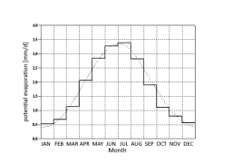
Annual pattern of potential evaporation according to /BRANDT, 1979/
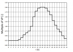
Daily pattern of potential evaporation as a multiple of the mean daily evaporation


Surface Water Storage (Impermeable Areas) O
For impermeable areas, snow storage and infiltration can be neglected, so that the balance equation is simplified as follows:
[math]\displaystyle{ N_W(t)=N(t)-VP(t)-\frac{dO}{dt} }[/math]
The change in surface water storage [math]\displaystyle{ dO/dt }[/math] represents the wetting of the surface as well as the filling and emptying (by evaporation) of depressions.

The following default value [math]\displaystyle{ BV }[/math] is used as wetting loss for impermeable areas.
[math]\displaystyle{ BV = 0.5 \mbox{ mm} }[/math]
Depression losses (MV) are specified by the user. The default and simultaneously maximum value in the model is 4 mm. Depression losses represent an average value for an sloped surface. Since depressions are not evenly distributed and runoff already begins before all depressions are completely filled, it is assumed that
- 1/3 of the impermeable area has a reduced depression loss of 1/3⋅MV
- 1/3 of the impermeable area has the average depression loss of MV
- 1/3 of the impermeable area has an increased depression loss of 5/3⋅MV
Therefore, runoff already occurs when the precipitation reduced by the evaporation rate exceeds the wetting loss and 1/3 of the depression losses (in case of dry starting conditions). The assumptions described above are shown as a schematic in the following figure.
The runoff coefficient of the impermeable areas (after covering the initial losses) is set at [math]\displaystyle{ \Psi = 1 }[/math]. When determining the portion of impermeable areas for a sub-basin, you must take into account that not all paved or sealed surfaces actually drain into a sewer system. The continuous provision of wetting and depression losses is achieved by continuously balancing the corresponding storages and the evaporation.
Surface Water Storage (Permeable Areas) O
The surface water storage of permeable areas is calculated by balancing a loss storage depending on the selected runoff generation approach. Details can be found in the following sections on the calculation of infiltration and runoff-effective precipitation.
Infiltration and runoff-effective precipitation I(t), NW(t)
In the case of permeable areas, infiltration into the soil cannot be neglected, since this has a decisive influence on the runoff. For the calculation three approaches are implemented in the model:
- Constant discharge coefficient [math]\displaystyle{ \Psi }[/math]
- Event-specific discharge coefficient based on the Soil-Conservation-Service (SCS) method
- Soil moisture simulation
Constant discharge coefficient Ψ
If a [math]\displaystyle{ \Psi }[/math] value is given, the remaining part of the precipitation after covering the initial losses (wetting and depression losses) is converted to runoff by multplying with [math]\displaystyle{ \Psi }[/math], independent of the antecedent conditions and the characteristics of the rainfall event (amount, intensity, duration). If possible, this approach should be avoided, since the process of runoff formation is greatly simplified.
Event-specific discharge coefficient based on the Soil-Conservation-Service (SCS) method
Using a CN value that is dependent on the soil type and land use (see /DVWK, 1991/), the initial losses and a relationship between the runoff coefficient and the accumulated rainfall amount up to the current point in time can be derived, both of which are dependent on antecedent conditions /Zaiss, 1987/. With this approach, the runoff coefficient increases with increasing precipitation amount during the course of the rainfall event. The quantification of the antecedent conditions is based on the 21-day-precipitation index [math]\displaystyle{ VN }[/math].
[math]\displaystyle{ V_N=\sum_{j=1}^21 C(j)^j \cdot hN_j }[/math]
with:
| [math]\displaystyle{ hN_j }[/math]: | Precipitation amount of the j-th previous day |
| [math]\displaystyle{ C(j) }[/math]: | Factor describing the influence of the j-th previous day |
The impact of different seasons is represented by an annual pattern of the factor C.
[math]\displaystyle{ C=0.05 \cdot \sin\frac{2\pi}{365}(i+0.75)+0.85 }[/math]
with:
| [math]\displaystyle{ i }[/math]: | current day of the hydrological year |
As a result, the value of C ranges between 0.8 < C < 0.9. This ensures that different rainfall indices are calculated for the same amount of rainfall at different times of the year, thus taking into account different degrees of runoff readiness. Depending on the antecedent conditions quantified in this way, a current discharge coefficient can be calculated using the CN values specific to the area and valid for average previous conditions. The following figure shows how the current discharge coefficient for different CN-values changes depending on antecedent conditions. Since the runoff readiness of a catchment area changes during the course of a rainfall event due to soil moistening, the runoff coefficient is also adjusted during an event as a function of the cumulative precipitation amount.
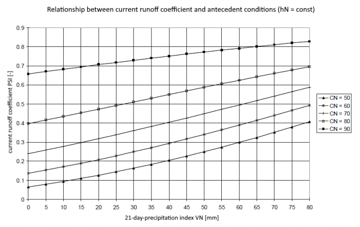
Dependence of the runoff coefficient on antecedent conditions
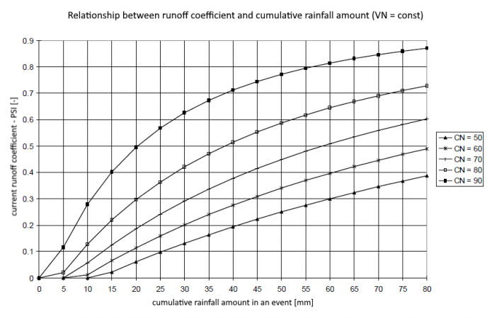
Dependence of the runoff coefficient on the cumulative precipitation sum


Soil Moisture Simulation
Land Use
When using soil moisture simulation, it is necessary to specify the land use. From the information about land use, the rooting depth is needed to determine the thickness of the root layer. Further parameters of land use, which are used to calculate interception and transpiration, are
- Root depth
- Coverage
- Annual pattern of coverage
- Leaf area index
- Annual pattern of the leaf area index
Haude factors entered as annual patterns can be assigned to each land use for a better consideration of the evaporation.
Soil Type / Soil Texture

The soil moisture simulation is based on a non-linear calculation of the individual soil layers. The soil is divided into different layers. Each layer is calculated individually and inflows and outflows reconciled with the layers below or above (if present). The following physical soil parameters are used as parameters for the soil moisture calculation:
- Wilting point (WP)
- Field capacity (FC)
- Total pore volume (TPV)
- Saturated conductivity (kf value)
- Maximum infiltration capacity (max. inf.)
- Maximum rate of capillary suction (max. cap.)
- Soil categorization: sand, silt, clay
The possible number of soil layers ranges from a minimum of one to a maximum of six. Experience has shown that the best results are achieved with a division into three layers. For this reason, the entered layers are always internally divided into three simulation layers:
- Infiltration layer (standard thickness [cm] = 20)
- Root layer (minimum thickness [cm] = 5)
- Transport layer (minimum thickness [cm] = 5)
The calculation of soil properties for the simulation layers is done by weighting them according to the given original thicknesses of the layers. In case of saturated conductivity the calculation is based on the principle of maintaining the continuity of the flow. For vertical flow, the velocity v at a given flow rate in one simulation layer should have the same value due to the continuity of the flow. Thus, the hydraulic gradient is no longer constant.
[math]\displaystyle{ kf_V=\frac{\sum_{i=1}^n d_i}{\sum_{i=1}^n \frac{d_i}{k_i}} }[/math]
with:
| [math]\displaystyle{ d_i }[/math]: | proportional layer thickness of the respective original layer [mm] |
| [math]\displaystyle{ k_i }[/math]: | saturated conductivity of the respective original layer [mm/h] |
| [math]\displaystyle{ kf_V }[/math]: | saturated conductivity of the simulation layer [mm/h] |

The water balance equation for a soil layer is solved on the basis of the piece-wise linear representation of the process functions which influence soil moisture: infiltration, current evaporation (evaporation + transpiration), percolation, interflow and capillary suction. The input variable for evaporation and transpiration is determined from the potential evaporation. The equation to be solved is:
[math]\displaystyle{ \frac{dBF(t)}{dt}=Inf(t)-Perk(t)-Eva_{akt}(t)-Trans_{akt}(t)-Int(t)+Kap(t) }[/math]
with:
| [math]\displaystyle{ BF(t) }[/math]: | current soil moisture |
| [math]\displaystyle{ Inf(t) }[/math]: | infiltration into the soil |
| [math]\displaystyle{ Perk(t) }[/math]: | percolation (seepage) |
| [math]\displaystyle{ Eva_{akt}(t) }[/math]: | current evaporation |
| [math]\displaystyle{ Trans_{akt}(t) }[/math]: | current transpiration |
| [math]\displaystyle{ Int(t) }[/math]: | interflow |
| [math]\displaystyle{ Kap(t) }[/math]: | capillary suction |

Infiltration, percolation, evaporation, transpiration, interflow and capillary suction depend on the current soil moisture. In the simulation, this dependence is described by the following functions.
[math]\displaystyle{ Inf(BF(t))=a_v \cdot \left(GPV-BF(t) \right)^{1.4}+k_f }[/math] (Approach according to HOLTAN)
[math]\displaystyle{ Perk(BF(t)) = \begin{cases} 0, & BF(t)\le f_{PK} \cdot nFK + WP \\ k_f \cdot \left(\frac{BF(t)-(f_{PK} \cdot nFK +WP)}{GPV-(f_{PK} \cdot nFK +WP)} \right)^{exp,PK}, & BF(t)\gt f_{PK} \cdot nFK + WP \end{cases} }[/math]
- (mod. approach according to /OSTROWSKI, 1992/)
[math]\displaystyle{ Eva(BF(t)) = \begin{cases} 0, & BF(t)\le WP \\ f_{Eva} \cdot \left(\frac{BF(t)-WP}{GPV-WP} \right)^{exp,PK}, & BF(t)\gt WP \end{cases} }[/math]
[math]\displaystyle{ Trans(BF(t)) = \begin{cases} 0, & BF(t)\le f_{Trans} \cdot nFK + WP \\ f_{Trans} \cdot \left(\frac{BF(t)-(f_{Trans} \cdot nFK +WP)}{GPV-(f_{Trans} \cdot nFK +WP)} \right)^{exp,PK}, & BF(t)\gt f_{Trans} \cdot nFK + WP \end{cases} }[/math]
with:
| [math]\displaystyle{ a_v }[/math]: | infiltration factor according to HOLTAN (in Talsim-NG [math]\displaystyle{ a_v=1 }[/math]) |
| [math]\displaystyle{ k_f }[/math]: | coefficient of conductivity of saturated soil |
| [math]\displaystyle{ nFK }[/math]: | available water capacity ([math]\displaystyle{ nFK=FK-WP }[/math]) |
| [math]\displaystyle{ WP }[/math]: | wilting point |
| [math]\displaystyle{ FK }[/math]: | field capacity |
| [math]\displaystyle{ GPV }[/math]: | total pore volume |
| [math]\displaystyle{ f_{PK} }[/math]: | soil-dependent scaling factor of the percolation function |
| [math]\displaystyle{ exp,PK }[/math]: | soil-dependent curvature parameter of the percolation function |
| [math]\displaystyle{ f_{Eva} }[/math]: | soil-dependent scaling factor of the evaporation function |
| [math]\displaystyle{ f_{Trans} }[/math]: | soil-dependent scaling factor of the transpiration function |
| [math]\displaystyle{ exp,Trans }[/math]: | curvature parameter of the transpiration function |
These parameters are calculated internally. The user only has to specify the soil parameters kf, WP, FC and TPV. The soil processes is are solved using a component for the simulation of storage.
Hydrologic Response Units
When runoff generation is calculated using soil moisture simulation, the concept of hydrologic response units (HRUs) is applied. A catchment area is divided into a number of hydrologically homogeneous areas, i.e. areas of the same soil type and the same land use. For each hydrologic response unit there is exactly one assignment of land use and soil type. The discharge resulting from a hydrologic response unit is output from the sub-basin element to which the HRU belongs, i.e. all hydrologic response units release discharge with the same time delay, independent of their location within the sub-basin.
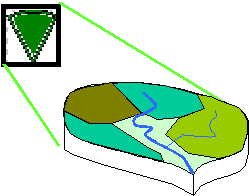
Division of a sub-basin element into hydrologic response units
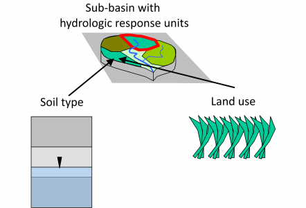
Assignment of soil type and land use to hydrologic response units


Runoff Concentration
Runoff concentration determines the delay of runoff from the catchment area. A parallel storage cascade with three reservoirs for permeable and one cascade for impermeable areas is used for surface runoff. The outflow of the components interflow and baseflow is output at the element outlet after passing through a single linear storage.
